Pediatric Pharmacometrics
Pharmacometrics, Pediactric drug development
If you have ever felt uncomfortable with pharmacometric analysis in pediatric patients, this page is for you, let’s walk through the basic concepts.
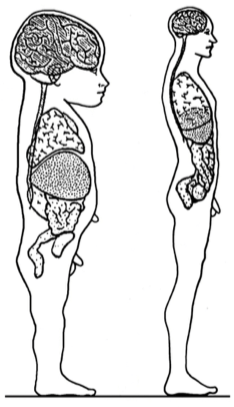
First things first: Children are not small adults. Children have quite different physiology (Figure 1), which must be taken into condsideration when evaluating PK and PD.
The differences in child–adult physiology can be further visualized through the arm-length/head-size ratio difference (See Video 1).
The age-related biological changes that occur as an individual matures from birth up to adulthood, is called ontogeny. The term ontogeny is especially used when talking about metabolic (enzyme) developement.
The use of model informed drug development (MIDD) approaches in pediatric drug development is highly recommended due to:
- Practical and ethical limitations in data collection.
- Ability to quantify the effects of growth and maturation by leveraging data from literature and older patients [1].
How do you measure the age of a child?
This is not as straight-forward as you might think! For everyday use, we would use the chronological age (i.e., time since birth). However, the development of a human begins well before birth. While the concept of when childhood begins is debated in social and ethical contexts (e.g., abortion), here we adopt the biological and regulatory definitions used in pediatric drug development.
Pediatric age terminology is commonly inconsistent. This is why it is important the be specific in how age is calculated. However, the terminology in Table 1 is generally accepted [2].
| Term | Abbreviation | Comment |
|---|---|---|
| Gestational (or “menstrual”) age | GA | Used when describing the age of a neonate. A 28-week, 5-day neonate is considered a 28-week neonate. |
| Postnatal (or “chronologial”) age | PNA | Time since birth |
| Postmenstrual age | PMA | Applied from 0–1 years of chronological age. A 33-week, 1-day GA infant who is 10 weeks, 5 days PNA would have a PMA of 43 weeks, 6 days. |
| Corrected (or “adjusted”) [gestational] age | CGA | Time since expected date of delivery (see Equation 1). Used to describe children up to 3 years of age who were born preterm. |
| Conceptional age | Time between conception and birth. Very accurate for in-vitro fertilization. |
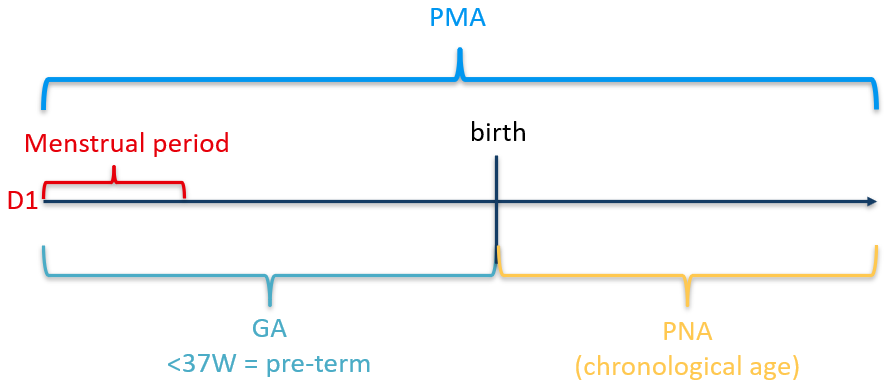
When patients are very young (< 1 year after birth), age is often related to the mothers last menstrual period. This is done because most women know when their last period began but not when ovulation occurred. This method of estimating the date of delivery is reliable as long as menstrual dates are remembered accurately (Figure 2).
Methods of determining GA should be clearly stated so that the variability inherent in these estimations can be considered when outcomes are interpreted. The convention for calculating GA when the date of conception is known is to add 2 weeks to the conceptional age. CGA is PNA reduced by the number of weeks born before 40 weeks of gestation (Equation 1).
Age groups
Age groups are to some extent arbitrary, but a classification such as the one in Table 3 provides a basis for thinking about study design. The identification of which ages to study should be medicinal product-specific and justified. Too many age groups might needlessly increase the number of patients required. Sometimes, it may be more appropriate to collect data over broad age ranges and examine the effect of age as a continuous covariate.
The study design and statistical plans should consider changing numbers of patients within a given age group, as patients grow older.
| Group | Age | Comment |
|---|---|---|
| Preterm neonates | birth–27 days (CGA, Equation 1) | < 39 weeks gestation |
| Term neonates | birth–27 days (CGA, Equation 1) | 39–41 weeks gestation |
| Infants | 28 days–23 months | |
| Children | 2–11 years | Often divided into 2–5 years, and 6–11 years. |
| Adolescents1 | 12–17 years | PK often similar to adults. |
| Adults | ≥ 18 years | Acts as reference. |
On the weight of children
One perhaps surprising fact is that neonates loose weight after birth, then regain it. Less surprisingly, females usually weigh less than males. Typical weight bands of children are:
| Age group | Weight (kg) | Comment |
|---|---|---|
| Preterm neonates | 0.5–4 | Using the Fenton growth chart [3] |
| Term neonates | 2.5–4.5 | |
| Infants | 5–15 | |
| Children | 15–30 | |
| Adolescents | 30+ | Approaching adult weights |
Pediatric PK studies
Relative bioavailability comparisons of pediatric and adult formulations should typically be done in adults. In contrast, PK studies in children are generally done in patients with the disease, warranting a clinically relevant dose to always be used.
For drugs with linear PK in adults, a single-dose study in pediatric patients may be sufficient for dose selection. with sparse sampling in multidose clinical studies to confirm the findings. However, when adults exhibit dose- or time-dependent PK or PD, pediatric steady-state studies become necessary.
Pediatric dosing is often expressed as mg/kg, up to the maximum adult dose. Although body surface area (BSA)-guided dosing might be preferred, it is often prone to measurement errors in height, particularly in infants and young children. Still, for medications with a narrow therapeutic window, such as many oncology drugs, BSA-guided dosing may be necessary.
PK extrapolation is often feasible
The feasibility of PK extrapolation is ultimately a clinical question. If an indication can be assumed to behave similarly in adult and pediatric populations, PK extrapolation (or “bridging”) can be used [4]. However, there could be cases in which a dedicated pediatric study is warranted (e.g., safety concerns or clinical presentation of the disease).
The relevant PK metric(s) linked to efficacy and safety and the exposure-response relationship should first be established in adults. As stated before, we want to start with a clinically relevant dose. The goal is to have pediatric exposure (not dose) comparable to that of adults.
The general procedure is to predict exposure in a pediatric age group (Table 3), collect data, refine predictions for the next younger group, and repeat. These models may be independent of adult models if there are adequate pediatric data, or they may be developed in combination with adult data.
See the EMA PIP QA (2025) for more information.
Allometric scaling
A previously developed adult PK model can be extrapolated to pediatric patients using allometry, which relates volume of distribution (
Below is a three-step guide on how to apply allometric scaling, inspired by Nathan Teuscher.
Step 1: Refit the final adult data with allometric exponents
Scale each volume parameter, including central volume and peripheral volumes.
Scale each clearance parameter, including total clearance (
Fix exponents if you don’t have pediatric PK data. Fix AND estimate them if you have pediatric PK data. Do a sensitivity analysis: How do the exposure predictions change?
The new model should give slightly different estimates for the volume and clearance parameters, but the diagnostics should be quite similar.
If your model already includes WT as a covariate, perhaps centered on the median WT instead of 70 kg, replace it with the standard allometric exponents Code 1, Code 2. Estimated exponents based on median WT can skew results when extrapolating beyond the observed range.
By converting to the standard WT of 70 kg and using standard exponent values, you rely on robust research when simulating outside adult data. Additionally, if AGE or WT is included elsewhere in the model, remove these covariates. They could cause problems with extrapolation after refitting the model with standard allometric exponents.
Maturation
In neonates, the maturation level of eliminating organs influences the estimates, and in adults, the body composition will affect them. Data from pediatric development programs are often too limited to confirm whether allometric exponents differ from theoretical values. EMA MWP (Methodology Working Party) considers the use of fixed exponents both scientifically justified and practical when developing popPK models in children.
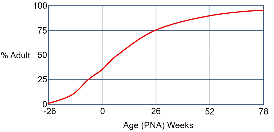
In lower ages (< 2 years), there are also maturation functions that come into play. For these pediatric patients, it is important to include maturation function(s) to describe pediatric PK. One maturation function is the Schwartz (bedside) formula (Code 3), where height is in cm, and SCr is in mg/dL.
But more commonly, the Rhodin formula is seen (Code 4).
The maturation half-life (TM50) is fixed to the literature value of 47.7 weeks and the Hill-exponent to the value of 3.4 [7]. The distribution (mean, [min–max]) of PMA (weeks) in this study population was (518, [57–1652]). Assuming renal maturation time differs in pre-term infants, a separate TM50 value could be estimated for them if the current model poorly describes this subgroup.
This is due to the high correlation between body weight and age in pediatric patients [8].
Step 2: Prepare a data set of pediatric simulation subjects
To generate pediatric simulation subjects, two main data sources are commonly used: NHANES (U.S. subjects, 2–18 years) and growth charts (e.g., WHO or CDC).
While NHANES provides individual-level subject data, its coverage of younger age groups is limited. This makes it less reliable for simulations involving infants or very young children. In such cases—typically for patients under 2 years of age—consider using growth charts.
Create at least 250 simulation subjects in each age group of interest (Table 3). You can adjust these age groups based on the disease condition or target patient population.
The growth charts provide the distribution of WT for various ages and statures of children. To create a simulation subject:
- Generate a uniform distribution of ages in each age-group, with the desired number of subjects.
- Create 250 simulated male subjects and 250 female subjects in the same age-group (e.g., 12–18 years).
- For each of these 500 subjects, identify the mean and standard deviation for
WTbased on their specificAGEandSEX. - Randomly sample a single
WTusing the mean and standard deviation from the growth chart.
This process creates a set of simulation subjects with WT, age group, and SEX.
Step 3: Simulate exposures and estimate target pediatric doses
Randomly sample ETAs (in e.g., R) to calculate the individual PK-parameters for each simulation subject. The WT will be used in the calculation of the
Adjust Dosepediatric,optimal to a feasible amount (Dosepediatric,adjusted). Rerun the simulations with the new dose and compare AUCpediatric,simulated to AUCadult,observed. It is expected that Dosepediatric,optimal will be different for each age group (Table 3).
How to present results from a PK extrapolation
The plot with all age groups receiving the adult clinical dose can be contrasted with a plot with age groups using Dosepediatric, adjusted. If you have pediatric data, you can overlay observed pediatric exposure with the simulated distributions to identify how well your model predicted the pediatric exposure.
The most relevant covariates influencing PK in pediatric patients is body weight accounting for size differences, and age (Figure 2) in the youngest pediatric patients to account for maturation of drug eliminating processes (see Code 4).
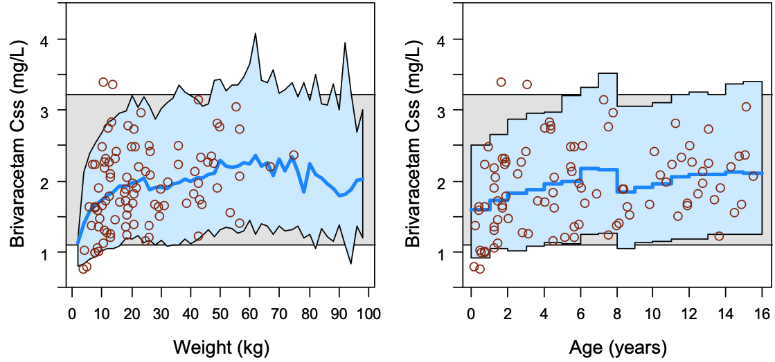
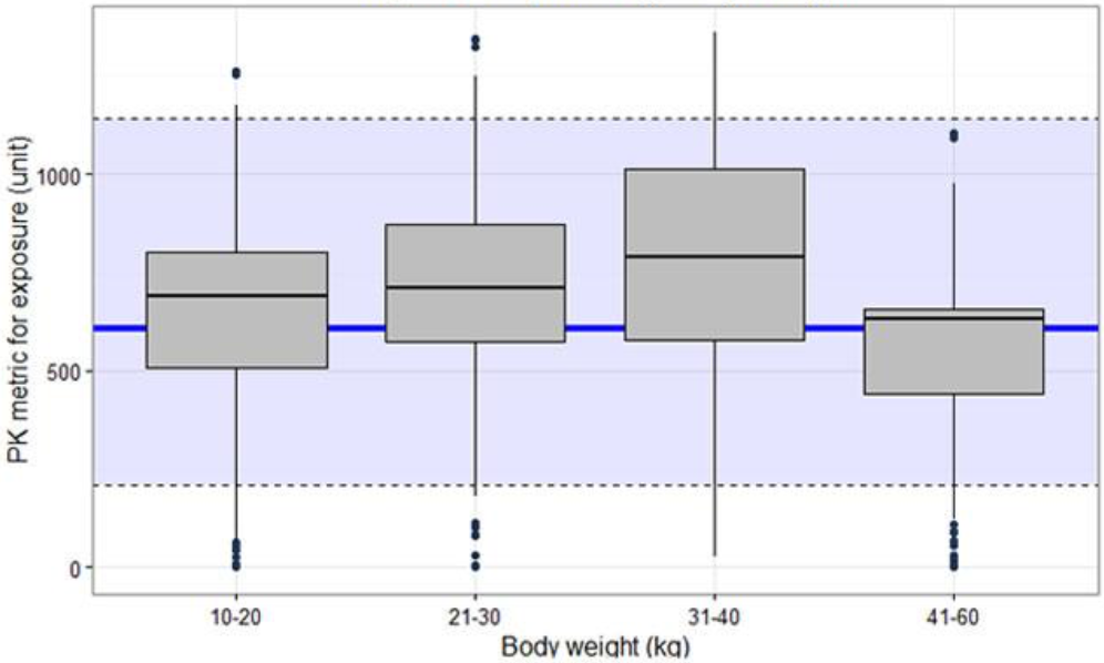
Relevant predefined exposure metrics should be presented graphically versus body weight and age on a continuous scale (Figure 4). If the drug is indicated to be used in the age range below one year, exposure vs body weight and age should be depicted in an additional separate figure focused on children 0–1 years.
Often plots that show the distribution of AUCpediatric,simulated along with the distribution of AUCadult,observed or simulated values from individual adult subjects using the final popPK model using box-plots can be useful (Figure 5). If different doses are proposed for bands of weight or/and age, exposure ranges predicted for the proposed doses for the subsets of the pediatric population should be visualized as box-plots (Figure 5). The reference range in the adult population (median and outer percentiles of observed or simulated data) should be given additionally (Figure 5). The same statistics should be presented numerically in tables.
See the EMA M&S QA (2023) for more information.
PD extrapolation is often not feasible
Unlike PK, PD models are disease- and therapy-specific, making direct extrapolation challenging. Thus, response (E-R) and PD models from adults may not apply to children.
Unless there’s clinical efficacy data in pediatric patients, be very cautious to extrapolate response or PD models from adults to pediatric patients.
Considerations include:
- Ontogeny of drug targets: Maturation of biological systems may alter response.
- Sensitivity adjustments: Use conservative parameters (e.g., lower EC50).
- Clinical caution: Without pediatric data, PD extrapolations are empirical.
One area where I have seen efficacy extrapolation being done is for bacterial infections. However, any PD extrapolation should always be discussed together with a medical expert.
References
Footnotes
Not the same as “teenager”! A teenager refers to chronological ages 13–19, while adolescent is a developmental age classification.↩︎
